Home Value Forecast
Measuring the Size of the Inventory of Distressed Real Estate: The Drain Is Still Clogged
One of the key questions about the current housing crisis is how the inventory of distressed real estate is affecting the path to recovery and the “new normal” for the housing market.
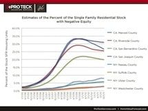
A variety of definitions of this distressed inventory have been offered. These definitions focus upon one of three components or stages of distress. One stage consists of those properties in which borrowers have negative equity and are facing the decision of whether or not to default on their mortgages. A second stage consists of properties that have gone into default and are facing the prospect of foreclosure. A third stage consists of properties in which foreclosure has already taken place and they are awaiting transition back to the market via an REO (real estate owned sale).
The purpose of this article is to introduce and discuss new measures of the size of this third stage generated by Home Value Forecast (HVF) and Collateral Analytics (CA).
Conventional Analysis Prior to the Current Crisis
As noted above, the conventional analysis of mortgage performance prior to the current crisis could be divided into three stages. Stage one focused primarily upon the decision to default, which involved the failure of a borrower to meet his or her mortgage obligations for a substantial period of time, typically 90 to 180 days delinquent. Analysis of vast amounts of data demonstrated that default was largely driven by the degree of negative equity associated with the property and, as a result, movements in the price of housing since the time of purchase or mortgage refinance.
Once the borrower defaulted, a second stage, the foreclosure process, began. This process involved “purchase” by the lender of the property, who usually “bid” the mortgage balance or whatever was owed the lender. State of the art models of mortgage foreclosure prior to the crisis would give some attention to state foreclosure laws because they influenced the time it took to go from a default to the foreclosure sale and this influences the ultimate cost of a default to a lender of a default. For example, the number of days between a default and the foreclosure sale was over 400 days prior to the crisis in New York and over 100 days in California. The primary reason for the difference was due to the processes used to permit a foreclosure sale. New York is a judicial foreclosure state and California is not.
The third stage of the process involved the sale by the lender in an arms-length sale to a third party, which are referred to as Real Estate Owned (REO) sales. Relatively little attention was given prior to the crisis to this stage of the process, which was effectively judged to be a stable and relatively unimportant determinant of future house price patterns and the pace of recovery of the broader housing market.
Properties in each stage of the process could be said to have been in some degree of distress. A possible headline of the current crisis is that the third stage has become a critical ingredient in any forecast on the pace of the housing recovery and the return to the “new normal”. The rise in the prominence of this dimension of the broader distressed inventory stems from the unprecedented growth in the number of foreclosures and the slow and uneven pace at which they are placed on the market to ultimately become REO sales.
HVF/CA’s Measure of the Stage 3 Distressed Real Estate Inventory
In this article, we introduce a new set of metrics developed by HVF and CA that focuses upon the size of the single family housing stock that has experienced a foreclosure sale and awaits return to the regular or nondistressed stock of single family housing via REO sales.
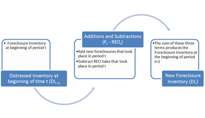
According to this measure, the size of the distressed inventory (DI) is measured by the number of single family properties that have been foreclosed upon but not yet sold by the lenders to a third party. It is measured as follows: DIt = DIt-1 + Ft – REOt, where Ft is the number of new foreclosure sales in period t and REOt is the number of REO sales in period t. This graphic below seeks to describe the measure. DI grows as the number of foreclosures increases and declines as the properties are sold as REOs.
Our interest is not only in the growth or decline of this measure of the distressed inventory but also in how it is influenced by changes in its two main components: new foreclosures and REO sales. We demonstrate the metrics using data for two sets of counties. One consists of four counties in Southern California. Another consists of four counties in downstate New York.
The average annual amounts of the Stage 3 distressed inventory are presented in Table 1 for years 2000 and 2005 thru 2011 for each of the eight counties. Simple averages of these measures are also presented by state and for all counties.

The averages of the four California and the New York counties are plotted in Figure 1.
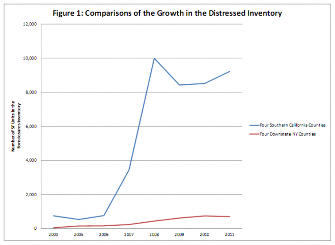
The most striking aspect of these measures is the rapid rise in the number of properties in the foreclosure inventory in California counties. The inventory is generally the largest in San Bernardino County during this period, which increased from about 1,500 properties in 2005 to nearly 16,000 in 2011:Q2. Though nearly a tenfold increase, the extent of the increase was even more pronounced in the other three California counties. For example, the distressed inventory increased from a mere 56 in 2005 to 1,576 in thru 2011:Q2. The size of the distressed inventories peaked in 2008 for three of the California counties but continued to grow throughout the entire period for San Bernardino County. The sizes of the distressed inventories peaked in 2010 for the New York Counties, and showed very modest declines through the second quarter of 2011.
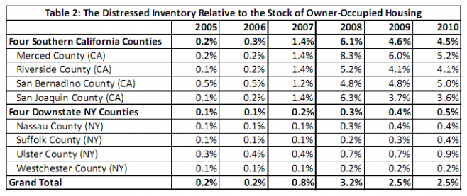
We adjust these data for the size of the stock of the owner-occupied housing with one or more mortgages. Data for the size of the housing stock are obtained from the American Community Survey for each of these counties for years 2005 thru 2010, the last year for which these data are currently available (See Table 2). The distressed inventory comprised between 4.8 and 8.3 percent of this stock of housing in the four California counties in 2008. The distressed inventory was a much smaller share of owner-occupied housing in New York and averaged 0.3 percent in 2008.
This measure of the distressed inventory provides an opportunity to focus upon its two main drivers or components: the rate of new foreclosures and the rate of exit from the inventory via REO sales. The first of these is depicted in Figure 2, which plots the annual average number of new foreclosures among the four California counties and the four New York counties.
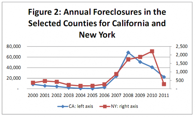
These averages are presented for two different scales to highlight the similarity in the trends in new foreclosures in the two groups of counties. Both rise steeply in 2007 and 2008. They continued to rise in 2009 and 2010 for the New York counties but did drop substantially in these years among the California counties.
The relatively rapid rise among the California counties once the crisis began is broadly consistent with the differences in the state foreclosure laws in these two states, as we would expect a faster increase in a nonjudicial state (California) than a judicial state (New York), all else equal. However, identifying a simple speed of adjustment from these data alone is quite difficult since foreclosure laws and policies that affect the speed of foreclosure have evolved during the crisis.
Beyond this relatively simple inference regarding state laws, these numbers alone cannot capture the myriad of law and policy changes since the start of the crisis. For example, the U.S. Treasury HAMP program is an obvious example of a national policy designed to promote loan modifications and avoid foreclosure. New York has also instituted two changes in its foreclosure laws since the start of the crisis to promote mortgage modifications via Judicial Settlement Conferences. California has remained a nonjudicial foreclosure state but a debate did take place about the potential for “dual tracking”, which refers to the possibility for a servicer to pursue both a foreclosure and a HAMP modification simultaneously.
Of course, the main reason for the difference in the rate of new foreclosures between the two sets of counties is that house prices declined much more substantially in the California counties than in the New York counties. Figure 3 highlights the trends in house prices for the two groups of counties.
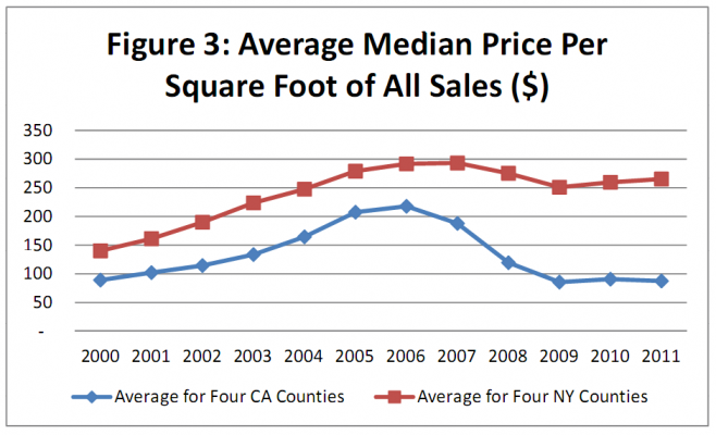
Again, the basic pattern is similar among the two groups: the median sale price per square foot of sales increased substantially from 2000 thru 2006 for both groups. The decline among the California counties begins a little sooner in New York and is much more pronounced. Indeed, prices by this metric are about the same in 2011 as they were in 2000 for the California counties. They remain above the 2000 values in 2011 among the New York counties.
The second major factor that we focus upon as a driver of the size of the Stage 3 distressed inventory is the rate at which properties exit the distressed inventory via REO sales. We measure this by examining the number of REO sales for each county and for years 2004 thru the second quarter of 2011. The higher the number of sales, all else equal, the faster the inventory dissipates.
The results are presented in Table 3.
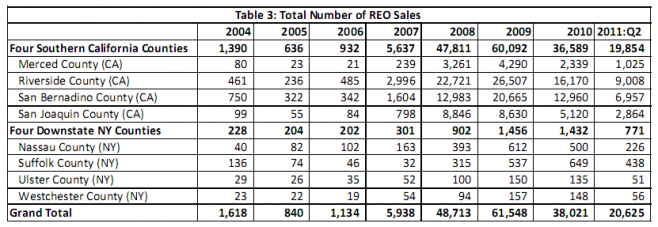
The main result is the wide variation in the number of REO sales during this time period. During the years in which the entry into the inventory by foreclosure sales was at its peak (2006 and 2007), the exit from the inventory via REO sales was at its low point, which contributed to the large increases in the Stage 3 distressed inventory. More recently, REO sales have increased by about ten times in California. They are about three times higher in the New York counties. These increases hasten the elimination of the foreclosure inventory.
Summary
The primary purpose of this article is to highlight new metrics developed by Home Value Forecast and Collateral Analytics to gauge the growth of what we call the Stage 3 distressed inventory and factors that affect its growth and decline. We associate the image of a drain to the Stage 3 distressed inventory. New foreclosures enter the drain and the drain is emptied by REO sales. The drain becomes clogged when the rate of new entries exceeds the pace of exits, which was the case in 2006 thru 2008. Though the pace of new foreclosures has declined and the pace of REO sales has increased, the drain is still severely clogged. This is especially apparent in the California counties.
In future writings we will address the harder question of how distressed inventory interacts with house prices. We will delve into smaller submarkets such as ZIP code since our sense is that the dominant impact of distressed real estate on house prices may be properties in close proximity to the distressed inventory. Stay tuned!
………………………………………………………………………………………………..
James R. Follain, Ph.D.
James R. Follain LLC and Advisor to FI Consulting
jfollain@nycap.rr.com
Norm Miller, PhD
Professor, Burnham-Moores Center for Real Estate
University of San Diego
nmiller@sandiego.edu
Michael Sklarz, Ph.D.
President
Collateral Analytics
msklarz@CollateralAnalytics.com
About Home Value Forecast
Home Value Forecast was created from a strategic partnership between SVI and Collateral Analytics. HVF provides insight into the current and future state of the U.S. housing market, and delivers 14 market snapshot graphs from the top 30 CBSAs.
Each month Home Value Forecast.com delivers a monthly briefing along with “Lessons from the Data,” an in-depth article based on trends unearthed in the data.
HVF is built using numerous data sources including public records, local market MLS and general economic data. The top 750 CBSAs as well as data down to the ZIP code level for approximately 18,000 ZIPs are available with a corporate subscription to the service. A demonstration is available upon request. Please visit the Contact Us page to request a demonstration.
To see how SVI and Collateral Analytics can help your company with its valuation needs, please contact us.